13 minutes read
It’s been a while since I’ve written an article on Data Science for Losers. A big Sorry to my readers. But I don’t think that many people are reading this blog. 
Now let’s continue our journey with the next step: Machine Learning. As always the examples will be written in Python and the Jupyter Notebook can be found here. The ML library I’m using is the well-known scikit-learn.
What’s Machine Learning
From my non-scientist perspective I’d define ML as a subset of the Artificial Intelligence research which develops self-learning (or self-improving?) algorithms that try to gain knowledge from data and make predictions based on it. However, ML is not only reserved for academia or some “enlightened circles”. We use ML every day without being aware of its existence and usefulness. A few examples of ML in the wild would be: spam filters, speech-recognition software, automatic text-analysis, “intelligent game characters”, or the upcoming self-driving cars. All these entities make decisions based on some ML algorithms.
The Three Families of ML-Algorithms
ML research, like any other good scientific discipline, groups its algorithms into different sub-groups:
- Supervised Learning
- Unsupervised Learning
- Reinforcement Learning
I think I should avoid to annoy you with my pseudo-scientific understanding of this whole subject so I’ll keep the definition of these three as simple as possible:
- Supervised Learning is when the expected output is already known and you want your algorithms to learn about relations between your input “signals” and the desired outputs. The simples possible explanation is: you have labelled data and want your algorithm to learn about them. Afterwards, you give the model some new, unlabeled data, and let it figure out what labels the data should get. It goes like this: Hey, Algorithm, look what happens (output) when I push this button (signal). Now learn from this example and the next time I push a “similar” button your should react accordingly.
- Unsupervised Learning is when you know nothing about your data, that is: no labels here, and let your favorite slave, Algorithm, analyze it to hopefully find some interesting patterns. It’s like: Hey Algorithm, I have a ton of messy (that is: unstructured) data. And because you are a computer and have all time in the world I’ll let you analyze it. In the mean time I’ll have a pizza and you’ll hopefully provide me some meaningful structure and/or relations within this data.
- Reinforcement Learning is in some way related to Supervised Learning because it uses so-called rewards to signal the algorithm how successful its action was. In RL the algorithm, the agent, interacts with the environment by doing some actions. The results of these activities are rewards which help the agent learn how well it performed. The difference between SL and RL is that these outcomes are not ultimate truths like the labelled data in SL, but just measurements. Therefore, the agent has to execute a certain amount of trial-and-error-tasks until it finds its optimum. It’s like: Hey Algorithm, this is the snake pit with pirate gold buried deep down. Now, bring it to me… 😈
In this article we’ll use the algorithms from the Supervised Learning family. And like any other scientific object the aforementioned families of algorithms are not the only grouping in Machine Learning. They’re, of course, much more granular and divided into sub-groups. For example, the SL family splits into Regression and Classification and then they split further into groups like Support Vector Machines, Naive Bayes, Linear Regression, Random Forests, Neural Networks etc. In general we have linear and non-linear methods to predict an outcome (or many of them). All of these methods are there to make predictions about data based on some other data (the training data).
Training the algorithms (Regression and Classification)
The data we analyze contains features or attributes (ordered as columns) and instances (ordered as rows). Just imagine you’d get a big CSV file with 100 columns and 1000.000 rows. The 99 columns define different attributes of this data set. For example, some DNA-information (genes, molecular structure etc.). And the rows represent different combinations of attributes which produce some outcome in an organism (for example, the risk of getting a certain disease). This result, the risk, is represented as a percentage ranging from 0% to 100%, in the 100th column. Now, your task would be to randomly take some of these rows, let’s say 800.000, and train your algorithm about the risks. The remaining 200.000 you keep separated from your training task so you can later use them to test how well your trained model behaves. Of course, the testing data would only contain 99 columns because it makes no sense to test your algorithm by giving it the already calculated outcomes (the 100th column). Simply spoken: you split the original data set into two sets each representing different time frames. The training data set represents the past and the testing data set represents the future data. You hope that based on past data your algorithm will be able to accurately predict the future (your testing data set for now) and all the upcoming data sets (the “real” future data sets). This ML model is based on Regression because we try to predict some ordered and continuous values (the percentages).
The ML models based on Classification are not calculating values but rather grouping instances of data sets into some predefined categories or classes, hence the name “classification”. For example, we could take a data set containing information about different trees and trying to predict a tree family based on certain attributes. Our algorithm would first learn what belongs to a certain tree family and try to predict it based on given attributes. Again, we’d split the original data set into two pieces, one for training the other for testing. Also, the testing part wouldn’t contain the information about the tree family (the class). The algorithm would then read all the attributes, row by row and calculate the possibility that a tree (the whole row) belongs to a certain family (one of the possible entries in the last column).
This is, in essence, what you’re doing when applying ML by using Supervised Learning. You have the data, you know about its form and quality of the results and now you want your algorithm to be trained so you can later use it to make predictions on data that will come later. In fact, you prepare your algorithm for the future based on the data from the past. Your ultimate goal is to create a model that is able to generalize the future outcomes based on what it has learned by analyzing some past data.
But, again, this article series is for Losers so we don’t care much about everything and focus ourselves on a few things we barely understand. 😳
A Classification Primer with sciki-learn and flowers
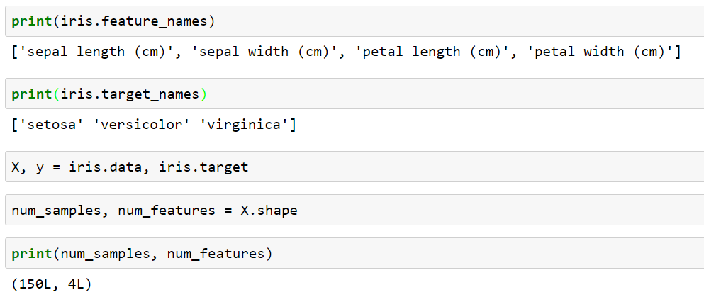
I’m pretty sure that the most of you already know the Iris data set. This data collection is very old and serves as one of standard examples when teaching people how to classify some data by providing a data set containing the attributes about the Iris flowers. In short, the Iris data set contains 150 samples (also called “observations”, “instances”, “records” or “examples”) about three different flower types (Iris setosa, virginica and versicolor). The instances are separated into four columns (or “attributes”, “features” , “inputs” or “independent variables”) describing sepal length & width, and petal length & width. Now the algorithm we’re going to use must correctly predict one of the possible outcomes (also called “targets”, “responses” or “dependent variables”): setosa, virginica or versicolor, represented by numbers 0, 1 and 2. Therefore: We have to classify the samples.
First we import scikit-learn and load the Iris data set. The Iris data set can either be loaded directly from scikit-learn or from a CSV file from the same directory where the notebook is located.
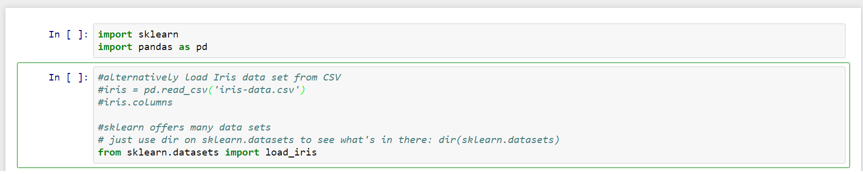
Scikit offers many different data sets. Just list them all by using dir(sklearn.datasets). All of them contain some general methods and properties:
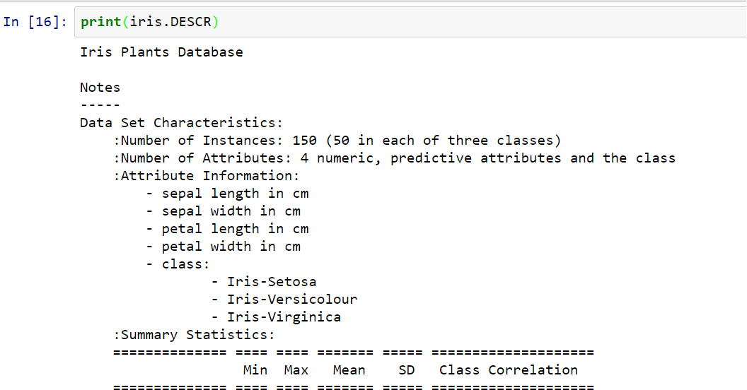
Here we see that our toy data set comprises of 150 instances (50 for each flower type), four attributes, which describe every single flower, and also the units used to calculate those values (centimeters in this case).
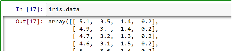
We can look into the raw data from Iris data set by using its data-property:
The respective targets (the classes we’ll try to predict) are also easily accessible:
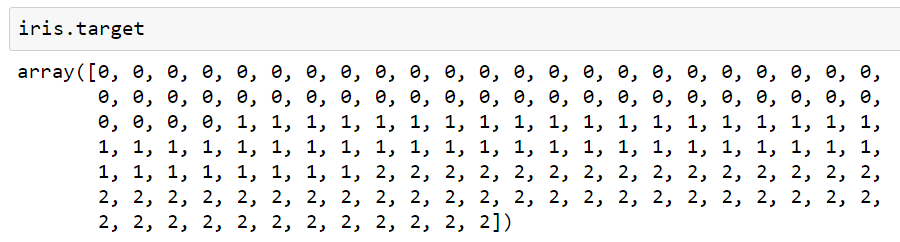
We see the distribution of the tree categories (classes) of flower types ranging from 0 to 2. The categories are represented as numerical values because scikit-learn expects them to be numerical.
As we see here the target array contains a grouped set of available categories. And this fact is very important because to create a proper training set we first must ensure that it contains a sound combination of all categories. In our case it wouldn’t be very intelligent to take only the first 60 entries, for example. The third flower category (numbered 2) wouldn’t be represented at all while the second one (numbered 1) wouldn’t be represented in a similar relation like in the original data set. Training our algorithm based on such data would certainly lead to biased predictions. Therefore we must ensure that all categories are correctly represented in the training data set. Also we should never let the whole data set be used for training the model because it would lead to overfitting. This means that our model would perfectly learn the structure of our testing data but will not be able to correctly analyze future data. Or, as you may often hear: the model would rather learn noise than signals.
Also, our decision of using Classification or Regression should not only be based on the shape of numerical values. Just because we see an ordered set of 0s, 1s and 2s doesn’t always mean we see categories here. Every time we want to develop a predictive model we have to learn about the explored data set first before we let the machine do the rest.
We gain additional information about our data set by exploring these properties (of course, in the wild we’d have to collect these names from different sources, like column names, documentation etc.):
It’s worth knowing that scikit-learn uses NumPy arrays to manage its data. These are, of course, much faster than traditional Python arrays.
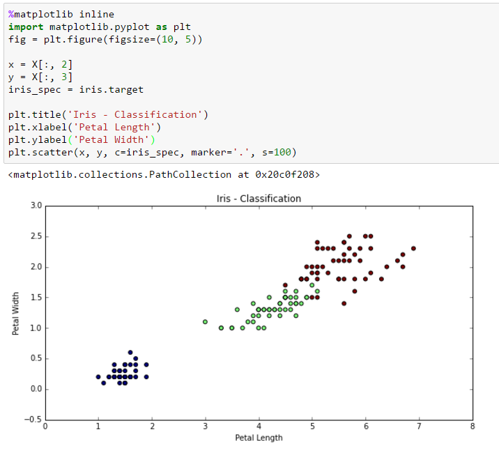
By using the excellent matplotlib package we can easily generate visual representations. Here we use petal length and and width as x respective y values to create a scatter-plot.
From X to y
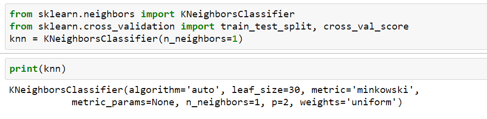
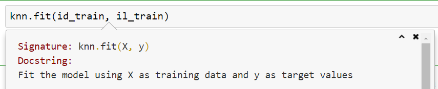
By convention the samples are located in a structure called X and their respective targets in y (small caps!). Both are NumPy arrays while the Iris data set is of type sklearn.datasets.base.Bunch. The reason we capitalize X is because of it’s structure: it’s a matrix while y is a vector. Hence, our work is based on a very simple rule: use X to predict y. Therefore, the learning process must be similar: give it X to learn about y. In this article we’ll use the k-Nearest Neghbor Classifier to predict the labels of Iris samples which will be located in the test data set. kNN is just one of many available algorithms and it’s advisable to use more than one algorithm. Luckily, the scikit-learn package makes it very easy to switch between them. Just import a different model and fit it to the same data set. There’s basically just one API to learn regardless of the currently used algorithm.
As already mentioned it’s very important to split data sets in such a way that no biased predictions occur. One of the possible methods is by using functions like train_test_split. Here we split our data into four sets, two matrices and two vectors:
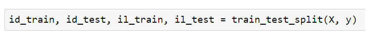
id stands for “iris data” (matrices) while il means “iris label” (vectors). We now use the training parts (which represent “data from the past”) to train our model.
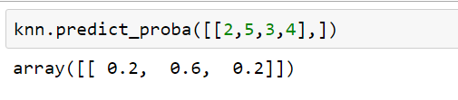
We can use our trained model to generate probabilistic predictions. Here we use some randomly typed numbers, which represent the four features, and let the model calculate percentages.
According to our trained model the chance of being setosa is at 20%, versicolor at 60%, and virginica at 20%.
Let’s test our trained model on some “future” data. In this case it’s the part we’ve got from the train_test_split function.
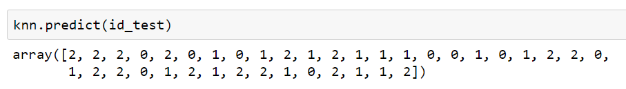
We see the predictions for each of the unlabeled samples. These are classes our model “thinks” the flowers belong to. Now let’s see what the real results are.
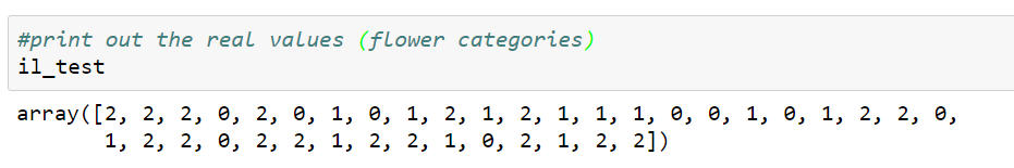
Compared the two with the naked eye we could say that the predictions were “OK” and mostly accurate. Here are the cross-validations scores:
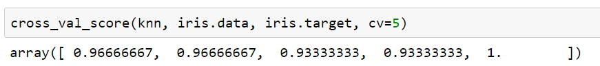
We see that our model is very accurate! Not bad for Losers like us. But this is mostly due to two simple facts: the Iris data set is only a “toy” data set and kNN is the simplest of all available algorithms.
Conclusion
I hope I could provide some “valuable” information regarding ML and how we can utilize algorithms from scikit-learn. This article should serve as a humble beginning of a series of articles on ML in general. In my spare time I’ll try to provide more examples with different algorithms (and will not use the iris data set and kNN again, I promise).