12 minutes read
Julia is what I’d like Python to be: dynamic but fast like C, supporting strong typing without being dogmatic (in both directions: static vs. dynamic), with a powerful REPL and many modules written in the same language (so I don’t have to switch to C). Julia is still a new language and I suppose not many of us use it currently in production. And yes, Julia is an ‘academic’ language, with a strong emphasis on technical/scientific computing, but honestly, would you rather like to run your business on an ‘anti-scientific’ / ‘anti-technical’ language? Yes, I know, it sounds very polemic because there are almost no such languages in widespread use (COBOL, I’m looking at you!). Of course, I’m still experimenting with Julia and watching all the nice videos, reading all the blogs, and everything else I can find on the net. Therefore, be warned: This article may contain false assumptions, silly code examples, or even blatantly stupid mistakes, but I feel strong obligation to give something back to the community. So many people helped me understand Julia better through their articles, videos and podcasts, so there’s no reason for a beginner like me to remain silent. Quite the opposite! Especially beginners should write more and encourage others to write about their experiences with Julia. All languages come into existence as projects of experienced teams and/or individuals but not a single language can survive without having a certain ‘critical mass’ of beginners. In that sense, this article is my brick.
As always, the sources are on GitHub.
The article is roughly split into three areas:
- general intro with usual examples on variables, loops, conditionals etc.
- introduction of some special Julia features like multiple dispatch and macros
- a few examples on DataFrames, DataArrays and Plotting with Julia
All examples are based on Julia v0.5.0-dev and run in a Jupyter 4.0 environment.
Julia with Jupyter
Julia comes with its own REPL that can be easily activated by typing julia in the console but I strongly recommend to give Jupyter a try. As you may already know Jupyter stands for (Ju)lia, (Py)thon and (R). Currently the stable version of Julia is 0.4.0 but I’ll be using the development branch 0.5.0. It depends on your preferences which branch you’d like to use. In both cases Julia’s package management would create separate subdirectories for compiled versions of modules we’ll be using throughout this article. Just for your information, this is how a console-based Julia-REPL looks like:

To use Jupyter you’ll need the IJulia package. To start a new notebook from Julia console type in:
using IJulia
notebook()
This will start a new notebook but block the console. Alternatively you can start the notebook with:
notebook(detached=true)
Now your console will remain accessible.
To start a notebook directly from DOS/Posix consoles just type in:
jupyter notebook

Then create a new notebook and select your local Julia compiler.

Like any other language, Julia has variables but unlike most other dynamic languages it infers the type of a value. Also, everything in Julia is an expression. Later we’ll see how this can help us create very powerful constructs by using meta-programming facilities.

Julia supports ASCII and UTF8/UTF16 Strings:

We can use tuples:

Arrays can be easily created but unlike many other languages they don’t start with index 0 but with 1.

An array can also be created by utilizing expressions. As we already know, everything in Julia is an expression, so a creation of an array can be a result of an expression:

Yet another way to create arrays is via ‘array comprehensions’. Many of you may have used similar techniques with Python. However, the types of these arrays are not the same. Above we have a StepRange while beneath we see a typical Array{Typename, Dimension} information.

Creating matrices in Julia is very convenient because it allows us to visually order the elements by rows and columns while separating them via semicolons. Here we see that the type of the array remained the same like in the last array while its dimension changed to 2. Of course, we can create as much dimensions as we need.

Conditionals are not a big surprise but take into account that Julia writes ‘elseif’ not ‘elsif’ or ‘else if’.

The ternary operator ? is also available:

Unlike many other languages Julia provides no switch/case/given statements or pattern matching (like in Scala, for example) but there are packages that provide such facilities.
The usual for-loop looks like this:

And the while-loop is like this:

Julia provides many useful macros (they always start with an @):

Accessing Julia’s help facilities is very easy: just prefix a term with a question mark.

Julia Functions
Julia is a functional language. This means that functions are first class objects and not just plain statements. You can assign them to variables, pass them as arguments or even return them as results (higher-order-functions). But, let’s begin with a simple example on how a Julia-function declaration looks like:

We use the keyword function followed by () that may contain parameters. Parameters can contain type information and this is always a better way to do it because with additional type information the Julia compiler can generate much faster code. If you don’t provide any type information then the compiler will generate all possible versions of a function and dispatch the ‘correct’ calls during the execution of the program. Later we’ll see how ‘multiple dispatch’ helps Julia to create powerful applications that combine the coding productivity of dynamic languages like Python together with raw speed of C.
Being a functional language Julia doesn’t expect you to explicitly write the return statement. If you don’t put a return in your function then the result of the last expression will be returned. As we already know everything is an expression in Julia so all functions will return a value.

A function can be written more concisely like this:

A function definition can be more specific by providing type information:

As already mentioned functions are treated like any other values. Therefore, we can return them to be used in some other part of the code. Note the definition of the returned function at the return statement: (a) -> aValue += a
We return an expression, not some generated value. Later we use this returned function to manipulate an ordinary value. In this case we simply double the original value.

Functions can be anonymous and accept arbitrary amount of arguments. In such cases just use the ‘splat’ operator …

When selecting the most specific version of a function Julia uses ‘multiple dispatch’. This means that it looks at the all of the available functions and its signatures and selects the one which has the most specific definitions of its signature according to the types of current arguments:. Here we can see which versions of a certain function are available in the current environment:

Unlike many other OO-languages methods have nothing to do with ‘instance functions’. Instead they describe the different versions of a certain function (in this case doubleIt). A function is an object in Julia and its methods are, well, ‘methods’. 😀
User-Defined Types
Julia neither has excessive class-hierarchies nor complex sub/super-typing. Instead, it offers a very thin, almost minimalistic user-defined-type handling. There are three ways to define a type:
- Abstract Types
- Mutable Types
- Immutable Types
Some general rules are:
- Abstract Types can’t contain any logic or fields.
- Mutable and Immutable Types can’t be subtyped.
- Immutable types can’t be changed.

In the last type iPhone we created a specialized version of its constructor by providing default values. The same technique can be used to create functions with default (or named) parameters.
Controlling & Introspecting Julia
Being a very open system and written almost completely in Julia there are lots of ways to check the own code or Julia’s internals. The two prominent macros are @code_llvm and @code_native
Just add the function call you’re interested in and Julia will provide you the generated code for LLVM and/or native assembly code of your architecture:

If you want to know how long it takes to execute a certain unction just use @time macro. Many Jupyter (IPython) users may remember the %timeit magic function.

User-Defined Macros in Julia
We can also write our own macros. To define a macro we have to use the macro keyword and declare its body with quote…end. Inside the body we can define what should happen and if there’ll be any interpolations (usually, we almost always interpolate certain expressions). The code parts that should be interpolated must begin with a $-sign.

Being a homoiconic language (like LISP) Julia treats its code and data the same way. Everything in Julia begins as a simple string and later gets parsed into an expression. This fact can be used to create very powerful constructs which can modify executing code. Many experiences Python programmers know how to utilize its meta-programming facilities.
here we create a function funcgen whose sole purpose is to iterate over a loop and each time execute @eval macro which will read the code after it as an expression and return new data as a result. In this case the complete definition of a function + its dynamically created name beginning with mult_ will become a part of the executing program.

Without the @eval macro the execution would simply stop with a syntax error. As we see Julia complains about invalid method names because it tried to execute a new function definition and failed to get a proper function name. Only with the @eval macro Julia can properly expand the expression starting with a $-sign.

After a successful exection we can immediately use the newly generated mult_ functions.

Accessing Data with Julia
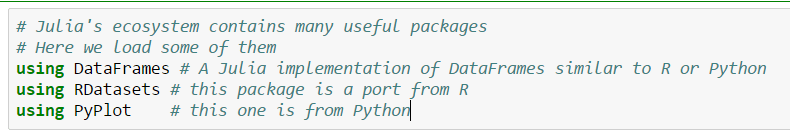
Julia offers many useful packages for different tasks. In this article we’ll focus on data and analysis. Of course, we’ll touch only a few simple parts of it but there should be no big barriers for those of you experienced with packages like R’s DataFrames or Python’s Pandas. Many libraries from R and Python are already available for Julia and there are many active projects busy with porting state-of-the-art packages from R and Python. In the following examples we’ll use R’s DataFrames / Datasets and Python’s PyPlot libraries. To be able to access PyPlot’s functionality you must have a properly installed Python version of it. To use a package in Julia you simply add a using statement together with the desired package name. If there’s no such package in your environment you can install it by using Pkg.add(PackageName) command. To update your environment simply execute Pkg.update() without any parameters.
After the packages have been successfully loaded we can use commands similar to those from the R-environment:

The port of the original R library contains many useful datasets:

We can use similar commands to get head, tail, describe etc.

We can group/count data very easily. Here we use the fifth column (the name of the species) and count the rows with function nrow.

We can also group by multiple columns like in this example with the ‘titanic’ dataset:

Working with data implies working with damaged, missing or wrongly formatter data. In such cases the standard arrays of Julia aren’t sufficient because they refuse to work with such data. to tackle such problems we use DataArrays and DataFrames. DataArrays are one-dimensional arrays capable of storing values like NA (not available):

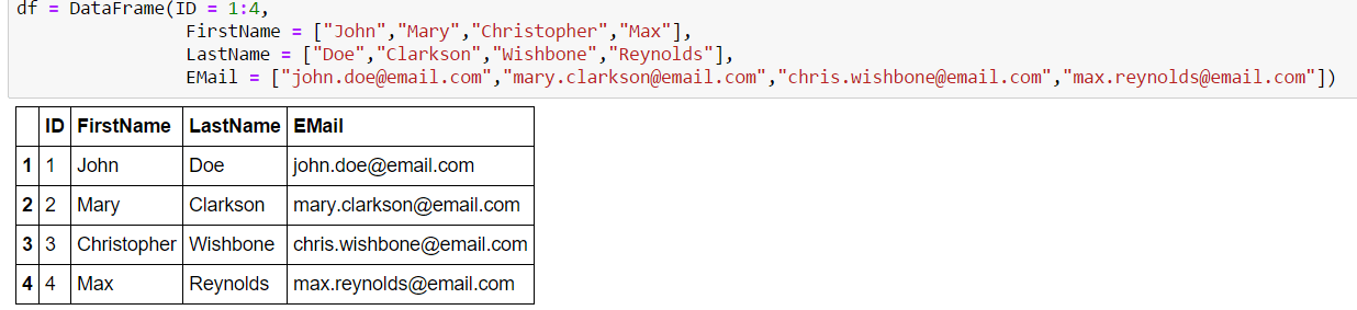
For 2-dimensional data like matrices (that is, tabular data) we can use DataFrames:
To visualize our data we can use different libraries like PyPlot, Gadfly etc. Here’s an example with Gadfly:

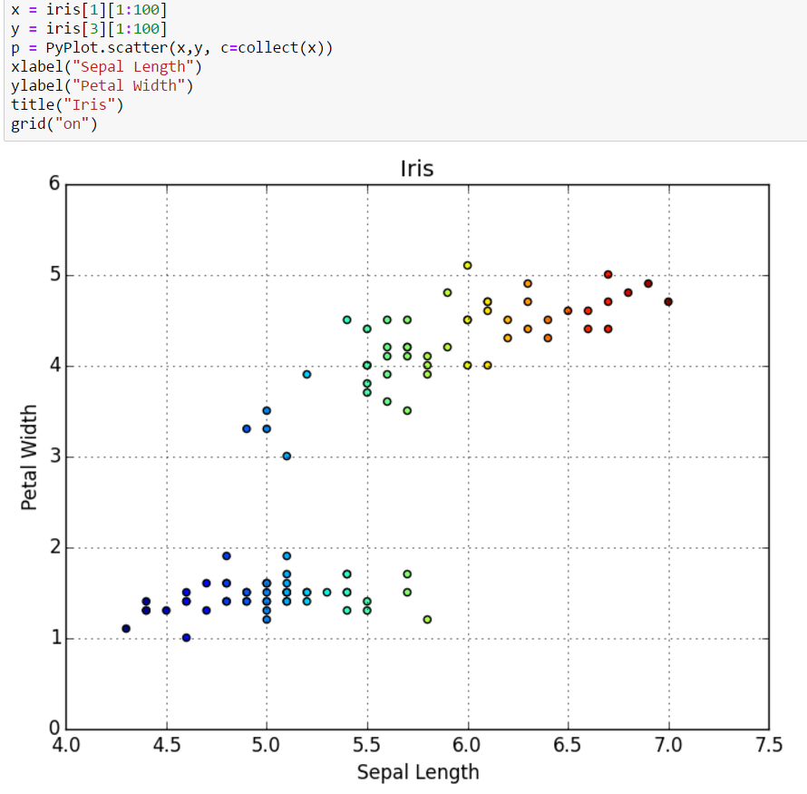
The well-known PyPlot library is also supported:
Conclusion
Julia is an exciting language that combined functionalities usually considered as ‘impossible’ to achieve. Either you go with a productive, dynamic language and sacrifice a lot of processing power, or you push the pedal to the metal by using C, C++, or Fortran while sacrificing a lot of programming productivity. But there never was a language that offered both of them without big sacrifices on any side. Julia seems to deliver such an environment and I hope I’ll soon get a chance to use it in production. Of course, this article only showed a few spots of a much bigger surface. For example, I’ve provided no examples on how easy it is to call external C or Fortran libraries. But there’ll be more articles on Julia in this blog. 😀


